Introduction to sampling

python

datacamp

statistics

machine learning

sampling

Author

kakamana

Published

January 8, 2023

Introduction to sampling

Get a better understanding of what sampling is and why it is so powerful. Additionally, We will learn about the problems associated with convenience sampling and what the difference between true randomness and pseudo-randomness is.

This Introduction to sampling is part of Datacamp course: Introduction to sampling

This is my learning experience of data science through DataCamp

Code

# Import seaborn with alias sns
import pandas as pd
import seaborn as sns
import numpy as np

# Import matplotlib.pyplot with alias plt
import matplotlib.pyplot as plt

Sampling and point estimates

Population: It is complete dataset
Sample: It is subset of data you calculate on

Population parameter: It is a calculation on population dataset Points vs. flavor: population pts_vs_flavor_pop = coffee_ratings[[“total_cup_points”, “flavor”]] np.mean(pts_vs_flavor_pop[‘total_cup_points’])

Point estimate: Or sample statistic is a calculation made on sample dataset Points vs. flavor: 10 row sample pts_vs_flavor_samp = pts_vs_flavor_pop.sample(n=10) cup_points_samp = coffee_ratings[‘total_cup_points’].sample(n=10) np.mean(cup_points_samp)

Simple sampling with pandas

The purpose of this exercise is to explore Spotify song data. There are over 40,000 rows in this population dataset, each representing a song. These columns include the title of the song, the artists who performed it, the release year, and attributes of the song, such as its duration, tempo, and danceability. To begin, you should examine the durations.

The Spotify dataset will be sampled and the mean duration of the sample will be compared with the mean duration of the population.

Code

spotify_population=pd.read_feather("dataset/spotify_2000_2020.feather")
spotify_population.head()

	acousticness	artists	danceability	duration_ms	duration_minutes	energy	explicit	id	instrumentalness	key	liveness	loudness	mode	name	popularity	release_date	speechiness	tempo	valence	year
0	0.97200	['David Bauer']	0.567	313293.0	5.221550	0.227	0.0	0w0D8H1ubRerCXHWYJkinO	0.601000	10.0	0.110	-13.441	1.0	Shout to the Lord	47.0	2000	0.0290	136.123	0.0396	2000.0
1	0.32100	['Etta James']	0.821	360240.0	6.004000	0.418	0.0	4JVeqfE2tpi7Pv63LJZtPh	0.000372	9.0	0.222	-9.841	0.0	Miss You	51.0	2000-12-12	0.0407	117.382	0.8030	2000.0
2	0.00659	['Quasimoto']	0.706	202507.0	3.375117	0.602	1.0	5pxtdhLAi0RTh1gNqhGMNA	0.000138	11.0	0.400	-8.306	0.0	Real Eyes	44.0	2000-06-13	0.3420	89.692	0.4790	2000.0
3	0.00390	['Millencolin']	0.368	173360.0	2.889333	0.977	0.0	3jRsoe4Vkxa4BMYqGHX8L0	0.000000	11.0	0.350	-2.757	0.0	Penguins & Polarbears	52.0	2000-02-22	0.1270	165.889	0.5480	2000.0
4	0.12200	['Steve Chou']	0.501	344200.0	5.736667	0.511	0.0	4mronxcllhfyhBRqyZi8kU	0.000000	7.0	0.279	-9.836	0.0	黃昏	53.0	2000-12-25	0.0291	78.045	0.1130	2000.0

Code

# Sample 1000 rows from spotify_population
spotify_sample = spotify_population.sample(n=1000)

# Print the sample
print(spotify_sample)

       acousticness                                            artists  \
7874        0.66400                                    ['The Walters']   
2664        0.01020                    ['Beastie Boys', 'Fatboy Slim']   
1683        0.00241                                          ['batta']   
14491       0.11400            ['AJ Mitchell', 'Ava Max', 'Sam Feldt']   
34495       0.96800                                         ['Yiruma']   
...             ...                                                ...   
25541       0.85400  ['Andrew Lloyd Webber', 'Patrick Wilson', 'Emm...   
904         0.71900                                   ['Carl Carlton']   
26932       0.02910                                    ['Cory Asbury']   
30144       0.14900                              ['Twenty One Pilots']   
12676       0.35000                                  ['Grupo Intenso']   

       danceability  duration_ms  duration_minutes  energy  explicit  \
7874          0.747     151683.0          2.528050   0.422       0.0   
2664          0.650     248507.0          4.141783   0.942       0.0   
1683          0.389     145400.0          2.423333   0.988       0.0   
14491         0.732     193548.0          3.225800   0.850       0.0   
34495         0.287     218293.0          3.638217   0.292       0.0   
...             ...          ...               ...     ...       ...   
25541         0.194     294160.0          4.902667   0.119       0.0   
904           0.546     153947.0          2.565783   0.828       0.0   
26932         0.572     333386.0          5.556433   0.685       0.0   
30144         0.550     277013.0          4.616883   0.625       0.0   
12676         0.718     219960.0          3.666000   0.529       0.0   

                           id  instrumentalness  key  liveness  loudness  \
7874   70QqoQ3krRFUHfEzit7vjT          0.002770  7.0    0.3920   -10.008   
2664   2WGGxhsc2WtPNkhsXWVcYb          0.000000  1.0    0.1220    -6.609   
1683   5V5akuBxKpIlTUPaueNpyy          0.000615  6.0    0.3460    -1.949   
14491  2wenGTypSYHXl1sN1pNC7X          0.000002  1.0    0.0388    -5.999   
34495  3xr8COed4nPPn6XWZ0iCGr          0.978000  9.0    0.0900   -19.285   
...                       ...               ...  ...       ...       ...   
25541  5klrh466oGToybceGHPGAX          0.000737  1.0    0.1090   -20.926   
904    5i7rT8lbGzjj1n7TTXR5U8          0.030000  4.0    0.3720    -4.771   
26932  0rH0mprtecH3grD9HFM5AD          0.000000  6.0    0.0963    -7.290   
30144  4IN3imzEuTsiHO6tOwDQu5          0.000000  1.0    0.1610    -8.213   
12676  0l7q7H1zYiJ9XHVqim2Uwc          0.000000  7.0    0.1510    -8.769   

       mode                                           name  popularity  \
7874    1.0                                   Goodbye Baby        55.0   
2664    1.0  Body Movin' - Fatboy Slim Remix/2005 Remaster        48.0   
1683    0.0                                          chase        61.0   
14491   1.0   Slow Dance (feat. Ava Max) - Sam Feldt Remix        72.0   
34495   1.0                             River Flows in You        62.0   
...     ...                                            ...         ...   
25541   1.0                               All I Ask Of You        57.0   
904     1.0                               Everlasting Love        48.0   
26932   1.0                                  Reckless Love        71.0   
30144   0.0                                       Trapdoor        56.0   
12676   1.0                                         Y Volo        45.0   

      release_date  speechiness    tempo  valence    year  
7874    2015-10-20       0.0294  111.141   0.5950  2015.0  
2664    2005-01-01       0.0754  101.786   0.7850  2005.0  
1683    2016-07-27       0.1070  111.975   0.0996  2016.0  
14491   2019-10-25       0.0444  124.024   0.3720  2019.0  
34495   2011-12-09       0.0541  145.703   0.3460  2011.0  
...            ...          ...      ...      ...     ...  
25541   2004-12-10       0.0398   85.698   0.1400  2004.0  
904     2009-01-01       0.0394  121.418   0.4010  2009.0  
26932   2018-01-26       0.0356  110.698   0.2320  2018.0  
30144   2009-12-29       0.0399  149.927   0.3170  2009.0  
12676   2001-10-16       0.0325  142.069   0.9440  2001.0  

[1000 rows x 20 columns]

Code

# Calculate the mean duration in mins from spotify_population
mean_dur_pop = spotify_population['duration_minutes'].mean()

# Calculate the mean duration in mins from spotify_sample
mean_dur_samp = spotify_sample['duration_minutes'].mean()

# Print the means
print(mean_dur_pop)
print(mean_dur_samp)
print("\n Notice that the mean song duration in the sample is similar, but not identical to the mean song duration in the whole population.")

3.8521519140900073
3.8048647333333334

 Notice that the mean song duration in the sample is similar, but not identical to the mean song duration in the whole population.

Simple sampling and calculating with NumPy

Code

# Subset the loudness column of spotify_population
loudness_pop = spotify_population['loudness']

# Sample 100 values of loudness_pop
loudness_samp = loudness_pop.sample(n=100)

# Print the sample
print(loudness_samp)

28889   -6.697
41542   -3.166
24096   -8.327
38021   -5.596
29360   -3.779
         ...  
34958   -7.206
41513   -7.560
28413   -7.113
41429   -6.073
38857   -4.433
Name: loudness, Length: 100, dtype: float64

Code

# Calculate the mean of loudness_pop
mean_loudness_pop = np.mean(loudness_pop)

# Calculate the mean of loudness_samp
mean_loudness_samp = np.mean(loudness_samp)

# Print the means
print(mean_loudness_pop)
print(mean_loudness_samp)
print("\n Again, notice that the calculated value (the mean) is close but not identical in each case")

-7.366856851353947
-7.385839999999999

 Again, notice that the calculated value (the mean) is close but not identical in each case

Convenience sampling

Collecting data by easiest method is convenience sampling

Sample bias: sample not true representation of population Selection bias

Are findings from the sample generalizable?

In your previous example, you saw that convenience sampling, which is the collection of data using the simplest method, can lead to samples that are not representative of the population. In other words, the findings of the sample cannot be generalized to the entire population. It is possible to determine whether or not a sample is representative of the population by examining the distributions of the population and the sample

Code

# Visualize the distribution of acousticness with a histogram
width = 0.01
spotify_population['acousticness'].hist(bins=np.arange(0,1.01,width))
plt.show()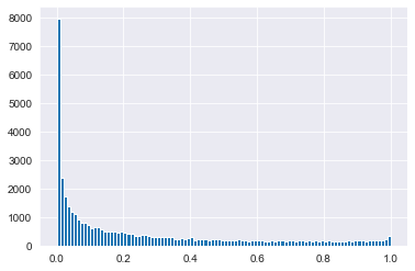

Code

spotify_mysterious_sample=spotify_population.sample(n=1107)
# Update the histogram to use spotify_mysterious_sample
spotify_mysterious_sample['acousticness'].hist(bins=np.arange(0, 1.01, 0.01))
plt.show()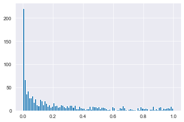

Code

# Visualize the distribution of duration_minutes as a histogram
spotify_population['duration_minutes'].hist(bins=np.arange(0,15.5,0.5))
plt.show()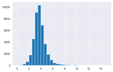

Code

spotify_mysterious_sample2=spotify_population.sample(n=50)
# Update the histogram to use spotify_mysterious_sample2
spotify_mysterious_sample2['duration_minutes'].hist(bins=np.arange(0, 15.5, 0.5))
plt.show()

Pseudo-random number generation

Code

# Generate random numbers from a Uniform(-3, 3)
uniforms = np.random.uniform(low=-3, high=3, size=5000)

# Print uniforms
print(uniforms)

# Plot a histogram of uniform values, binwidth 0.25
plt.hist(uniforms, bins=np.arange(-3,3.25,0.25))
plt.show()

[ 0.46978238 -1.66176314  1.31080161 ...  0.27384823  0.57683707
  1.94834767]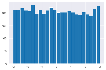

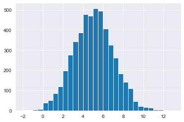
Code

# Generate random numbers from a Normal(5, 2)
normals = np.random.normal(loc=5,scale=2,size=5000)

# Print normals
print(normals)

# Plot a histogram of normal values, binwidth 0.5
plt.hist(normals,np.arange(-2,13.5,0.5))
plt.show()

[0.37088348 5.46510043 5.6804744  ... 5.06268094 7.1989964  4.26078515]